Public transport optimization research using Genetic Algorithms

Where a city puts its bus stops decides how far people walk, how much of the network they can actually use, and how much the operator spends. This research tackles that as a multi-objective optimization problem and answers it with an evolutionary algorithm, instead of collapsing everything into one score.

It started as the final project of the Evolutionary Algorithms course at the Universidad de la República (Uruguay) and grew into a paper with Sergio Nesmachnow (UdelaR) and Diego Rossit (Universidad Nacional del Sur, Argentina). It was presented at the Ibero-American Congress on Smart Cities (ICSC CITIES 2025) in Puebla, Mexico, and an extended version was published in Frontiers in Future Transportation.

The problem

Each census segment can get no stop or one of three stop qualities (basic, simple shelter, double shelter). Three goals pull against each other:

Maximize coverage: the demand-weighted number of trips whose origin and destination are both within reach of a stop.
Minimize the number of stops: a proxy for bus dwell time, and therefore travel time.
Minimize cost: installation cost by stop type, weighted by local demand so that building in low-demand areas is penalized.

Adding stops raises coverage but also cost and travel time, so there is no single best answer. That is why the output is a Pareto front.

The fitness function

The model is defined over the set $|S|$ of census segments, which double as candidate stop locations, and the set of stop types $T=\{0,1,2,3\}$ (none, basic, simple shelter, double shelter). The decision variable $y_{ts}$ is 1 when segment s gets a stop of type t, and $z_s$ is 1 when s is covered, meaning at least one stop exists inside its coverage neighborhood $N(s)$ . A trip counts as covered only if both its origin and destination are covered.

Three objectives

This is the fitness vector the multi-objective algorithm evaluates directly, with no weights:

\begin{aligned}\max f_{cov} &= \sum_{o \in S}\sum_{d \in S}\bigl(trips_{od}+trips_{do}\bigr)\, z_o z_d \\[4pt] \min f_{stops} &= \sum_{i \in S}\sum_{t \in T} y_{it} \\[4pt] \min f_{cost} &= \sum_{i \in S}\sum_{t \in T} c_t \left(\frac{\sum_{o \in S} trips_{oi}+\sum_{o \in S} trips_{io}}{D^{max}}\right) y_{it}\end{aligned}

Coverage sums the trips in both directions between every pair of covered segments.
Stops counts the installed stops.
Cost adds the cost $c_t$ of each installed stop, scaled by how busy its segment is relative to the busiest pair in the city, $D^{max}$ , defined as:

D^{max}=\max\{trips_{od}+trips_{do}\mid \forall o,d \in S\}

Constraints

\begin{aligned}\sum_{t \in T} y_{it} &= 1, && \forall i \in S \\[4pt] z_i &\le \sum_{s \in N(i)}\sum_{t \in T\setminus\{0\}} y_{st}, && \forall i \in S \\[4pt] |N(i)|\, z_i &\ge \sum_{s \in N(i)}\sum_{t \in T\setminus\{0\}} y_{st}, && \forall i \in S \\[4pt] z_i,\, y_{it} &\in \{0,1\}\end{aligned}

Each segment gets exactly one stop type (type 0 means no stop). A segment is covered if and only if some segment in its neighborhood has a stop of type 1 to 3. All variables are binary.

Normalized fitness for the single-objective baselines

The single-objective GA and the local search need one number to compare solutions. Each objective is rescaled to $[0,10]$ and then combined with weights. Coverage is divided by its theoretical maximum $COV^{max}$ (the sum of all demand):

f'_{cov}=\frac{f_{cov}}{COV^{max}}\times 10

The stop count is normalized by the number of segments:

f'_{stops}=\frac{f_{stops}-|S|}{|S|}\times 10

Cost is normalized between its minimum and maximum achievable values $C^{max},\, C^{min}$ . The bracketed demand factor in c_i runs from $-1$ in the highest-demand segments (building there is rewarded) to $+1$ in the lowest-demand ones (building there is penalized):

\begin{aligned}f'_{cost}&=\frac{C^{max}-\sum_{i \in S} c_i}{C^{max}-C^{min}}\times 10 \\[6pt] c_i&=\sum_{t \in T} c_t\, y_{it}\left[2\left(1-\frac{\sum_{o \in S} trips_{oi}+\sum_{o \in S} trips_{io}}{D^{max}}\right)-1\right]\end{aligned}

The final fitness is the weighted sum:

F(s)=w_{cov}\, f'_{cov}+w_{stops}\, f'_{stops}+w_{cost}\, f'_{cost}

The weights $w_{cov},\, w_{stops},\, w_{cost}$ were set with a grid search over five candidate values per weight, 125 combinations in total, favoring coverage while still pushing toward cheaper, better-placed stops. The multi-objective algorithm skips this step entirely, which is why it can return the whole trade-off curve instead of one weighting of it.

How it works

How the pieces fit together: demand data goes in, an integer-encoded population evolves under three competing objectives, and a Pareto front comes out.

The solver is a customized NSGA-II on top of jMetal. The operators are tailored to the stop-type encoding: two-point crossover, an integer mutation that prefers moving a gene to an adjacent stop type, and an initialization that favors empty segments with a few high-quality stops as seeds. Coverage masks are precomputed per candidate and updated incrementally, which is what keeps city-scale evaluation fast.

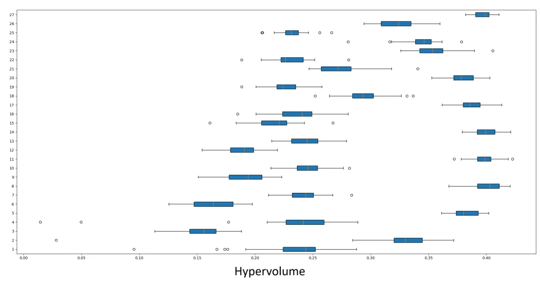
Parameters were tuned on a separate instance (Pittsburgh, 4,100 candidate locations) so the evaluation cities stayed unseen. All 27 combinations of population size, crossover and mutation probability were run 30 times each and compared with ANOVA on relative hypervolume. The winner (population 200, crossover 0.8, mutation 0.1) was used for every experiment.

Box plots of relative hypervolume for the 27 parameter configurations — Relative hypervolume for the 27 parameter configurations, 30 runs each. Configuration #27 scored best.

Results

A far better Pareto front than a single-objective GA

The baseline is a single-objective GA with the same operators and weighted-sum fitness, tuned with a 125-combination grid search over the weights. Metrics are computed against a reference front built from 30 independent runs.

Montevideo	MOEA	GA
Pareto-optimal solutions (higher is better)	208	18
Error ratio (lower is better)	0.000	0.640
Generational distance (lower is better)	0.000	0.036
Spread (lower is better)	0.239	0.714
Relative hypervolume (higher is better)	0.992	0.209

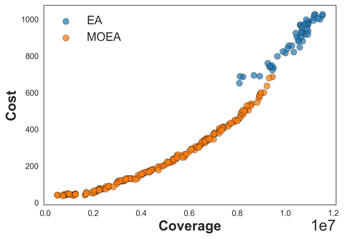
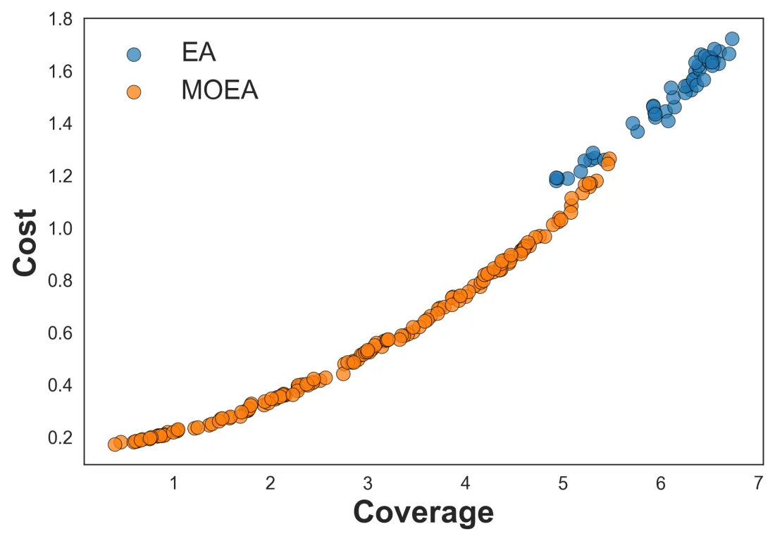
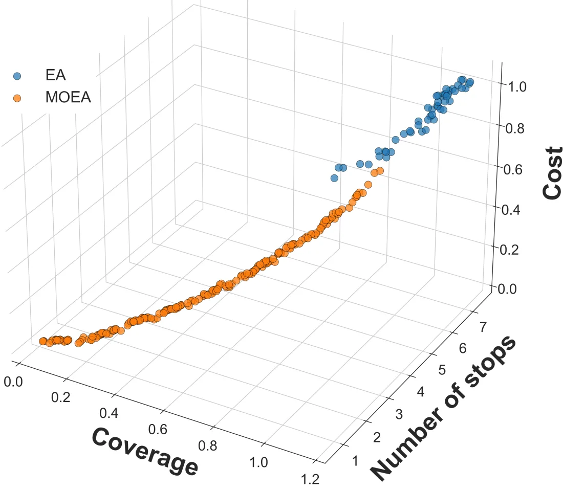
Buenos Aires shows the same pattern (relative hypervolume 0.990 vs 0.178). The plot below shows why: the single-objective GA only samples the expensive, high-coverage corner, while the MOEA covers the whole trade-off curve and dominates the GA wherever the two overlap.

Pareto front for Montevideo, coverage versus cost, MOEA against single-objective GA — Montevideo: coverage vs. cost.

Pareto front for Buenos Aires, coverage versus cost, MOEA against single-objective GA — Buenos Aires: coverage vs. cost.

Three-dimensional Pareto front for Montevideo over coverage, number of stops and cost — The full three-objective front for Montevideo (normalized axes).

A more cost-effective compromise than local search

Taking the compromise solution from each method, and using coverage per unit of cost as a common yardstick:

Method	Stops	Cost	Coverage / cost
MOEA (compromise)	317	248	23,352
Single-objective GA	527	652	12,395
Local search	987	733	16,677

Local search covers the most trips in absolute terms, but only by putting a stop in every one of the 987 segments. The MOEA compromise uses 68% fewer stops and about 66% less cost, and improves the coverage-to-cost ratio by 46.9% over local search and 28.6% over the single-objective GA.

What the solutions look like on a map

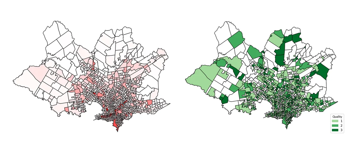
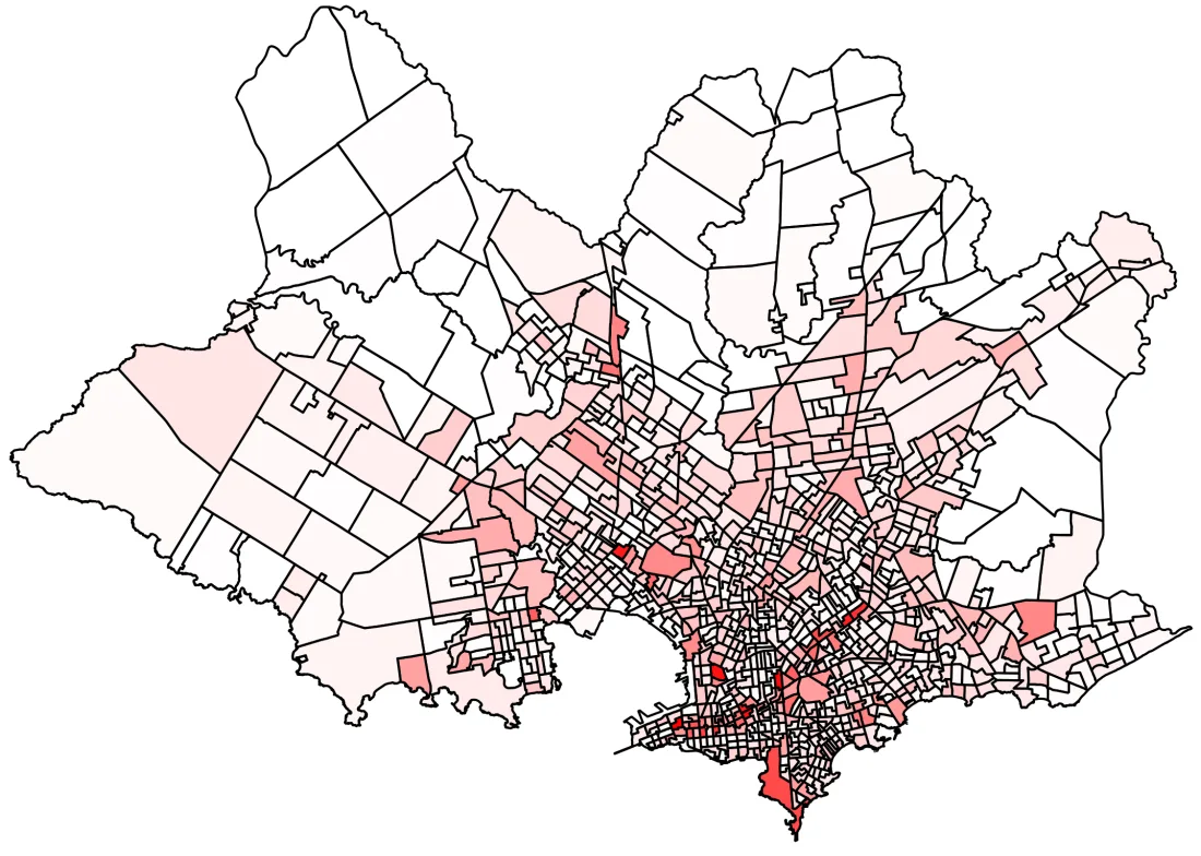
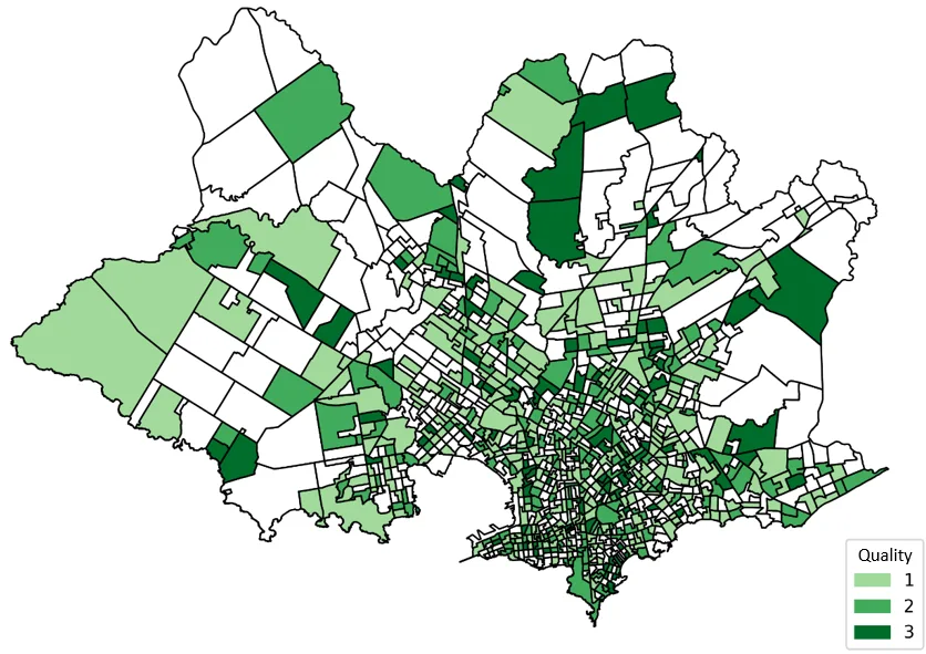
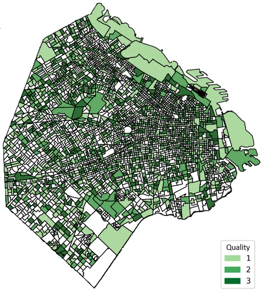
The compromise solution follows demand without being told where the city center is: premium stops cluster in the dense center and along main corridors, peripheral segments get lighter infrastructure, and low-demand segments are served by anchor stops in neighboring segments instead of getting their own. The result is a hierarchical, backbone-shaped network.

Map of Montevideo census segments shaded red by transit demand — Montevideo. Left: demand per census segment (darker is higher). Right: stop quality assigned by the best-trade-off solution (1 basic, 2 shelter, 3 double shelter).

Map of Montevideo census segments shaded green by assigned stop quality — Montevideo. Left: demand per census segment (darker is higher). Right: stop quality assigned by the best-trade-off solution (1 basic, 2 shelter, 3 double shelter).

Map of Buenos Aires census segments shaded green by assigned stop quality — Buenos Aires: the same method on a much larger instance. High-quality stops concentrate in the center and along the coast.

Takeaways for planners

Hand over options, not a verdict: a Pareto set lets decision makers pick by budget, politics or service goals, and shows how much one objective costs in another.
Equity needs explicit rules: cost-efficient solutions favor dense areas, so periphery protection should be added as a constraint or objective.
Re-optimize as demand shifts: runs finish in under half an hour, which makes "what if" studies practical.

Future work covers demand uncertainty, equity indicators and budget constraints, and walking-distance and network-based coverage.

Resources

Journal article, Frontiers in Future Transportation (2026): Read the paper.
Repository: GitHub repo (Java, jMetal, Maven, with the plotting scripts).
Certificate of participation, ICSC CITIES 2025: View certificate.